Case study: Babynames
This dataset is available from Kaggle. We are going to use this dataset to demonstrate some of the steps that you might have to take in order to transform a raw dataset into what you need to do in order to do the analysis that you are planning.
1 Importing data
Here we read the CSV file into the babynames data frame.
2 Examining data
Now let’s take a look at what we have:
  YearOfBirth       Name               Sex                Number
 Min.   :1880   Length:1858689     Length:1858689     Min.   :    5.0
 1st Qu.:1950   Class :character   Class :character   1st Qu.:    7.0
 Median :1983   Mode  :character   Mode  :character   Median :   12.0
 Mean   :1973                                         Mean   :  183.4
 3rd Qu.:2002                                         3rd Qu.:   32.0
 Max.   :2015                                         Max.   :99680.0
As you can see above, there are more than 1.8 million observations (rows) in this dataset. How many babies are represented within this dataset?
Over 340 million!
Let’s look at the top 15 rows of babynames, ordered alphabetically within YearOfBirth and Sex. We would expect to see names for females beginning with A from 1880:
   YearOfBirth     Name Sex Number
1         1880    Abbie   F     71
2         1880     Abby   F      6
3         1880  Abigail   F     12
4         1880      Ada   F    652
5         1880     Adah   F     24
6         1880  Adaline   F     23
7         1880     Adda   F     14
8         1880    Addie   F    274
9         1880    Adela   F      9
10        1880 Adelaide   F     65
11        1880    Adele   F     41
12        1880   Adelia   F     18
13        1880  Adeline   F     54
14        1880   Adella   F     26
15        1880   Adelle   F      5
Now we can reorder these rows descending by Number within YearOfBirth and Sex—that is, for each year and gender, it will list the names from most popular to least popular.
3 Modifying and calculating
We are going to do some calculations on the datatable. For each YearOfBirth and Sex, we want to calculate how many names are recorded that year and how many babies are in the dataset. In the first observation, you can see that 90,992 female babies are given 942 names in 1880.
BabyYearSex <-
  babynames |>
    group_by(YearOfBirth, Sex) |>
    summarize(
      NumOfNames = n(),
      NumOfBabies = sum(Number),
    )
head(BabyYearSex, n=8)
# A tibble: 8 × 4
# Groups: YearOfBirth [4]
YearOfBirth Sex NumOfNames NumOfBabies
<int> <chr> <int> <int>
1 1880 F 942 90992
2 1880 M 1058 110490
3 1881 F 938 91953
4 1881 M 997 100743
5 1882 F 1028 107848
6 1882 M 1099 113686
7 1883 F 1054 112318
8 1883 M 1030 104627Let’s use the slice() function to get the top names for each YearOfBirth/Sex combination.
babynames |>
  arrange(YearOfBirth, Sex, desc(Number)) |>
  group_by(YearOfBirth, Sex) |>
  slice(1:10) |>
  head(n=15)
# A tibble: 15 × 4
# Groups: YearOfBirth, Sex [2]
YearOfBirth Name Sex Number
<int> <chr> <chr> <int>
1 1880 Mary F 7065
2 1880 Anna F 2604
3 1880 Emma F 2003
4 1880 Elizabeth F 1939
5 1880 Minnie F 1746
6 1880 Margaret F 1578
7 1880 Ida F 1472
8 1880 Alice F 1414
9 1880 Bertha F 1320
10 1880 Sarah F 1288
11 1880 John M 9655
12 1880 William M 9531
13 1880 James M 5927
14 1880 Charles M 5348
15 1880 George M 5126Now that we know how to do it, let’s store that information in a data frame:
BabyYearTopNames <-
  babynames |>
    arrange(YearOfBirth, Sex, desc(Number)) |>
    group_by(YearOfBirth, Sex) |>
    slice(1:10)
head(BabyYearTopNames, n=15)
# A tibble: 15 × 4
# Groups: YearOfBirth, Sex [2]
YearOfBirth Name Sex Number
<int> <chr> <chr> <int>
1 1880 Mary F 7065
2 1880 Anna F 2604
3 1880 Emma F 2003
4 1880 Elizabeth F 1939
5 1880 Minnie F 1746
6 1880 Margaret F 1578
7 1880 Ida F 1472
8 1880 Alice F 1414
9 1880 Bertha F 1320
10 1880 Sarah F 1288
11 1880 John M 9655
12 1880 William M 9531
13 1880 James M 5927
14 1880 Charles M 5348
15 1880 George M 5126Let’s calculate how many babies are given one of the top names (for each sex) for each year:
# A tibble: 272 × 3
# Groups:   YearOfBirth [136]
   YearOfBirth Sex   CountTopBabiesThisYear
         <int> <chr>                  <int>
 1        1880 F                      22429
 2        1880 M                      48854
 3        1881 F                      22211
 4        1881 M                      44122
 5        1882 F                      25820
 6        1882 M                      48566
 7        1883 F                      26308
 8        1883 M                      44600
 9        1884 F                      29860
10        1884 M                      47180
# ℹ 262 more rows
Again, let’s now store this information in a data frame:
BabyYearTopNamesSums <-
  BabyYearTopNames |>
    group_by(YearOfBirth, Sex) |>
    summarize(
      CountTopBabiesThisYear = sum(Number))
head(BabyYearTopNamesSums)
# A tibble: 6 × 3
# Groups: YearOfBirth [3]
YearOfBirth Sex CountTopBabiesThisYear
<int> <chr> <int>
1 1880 F 22429
2 1880 M 48854
3 1881 F 22211
4 1881 M 44122
5 1882 F 25820
6 1882 M 48566Use left_join() to get all of the yearly statistics in one table:
BabyYearSex <-
  BabyYearSex |>
    select(YearOfBirth, Sex, NumOfNames, NumOfBabies) |>
    left_join(BabyYearTopNamesSums,
              by = join_by(YearOfBirth, Sex))
head(BabyYearSex, n=8)
# A tibble: 8 × 5
# Groups: YearOfBirth [4]
YearOfBirth Sex NumOfNames NumOfBabies CountTopBabiesThisYear
<int> <chr> <int> <int> <int>
1 1880 F 942 90992 22429
2 1880 M 1058 110490 48854
3 1881 F 938 91953 22211
4 1881 M 997 100743 44122
5 1882 F 1028 107848 25820
6 1882 M 1099 113686 48566
7 1883 F 1054 112318 26308
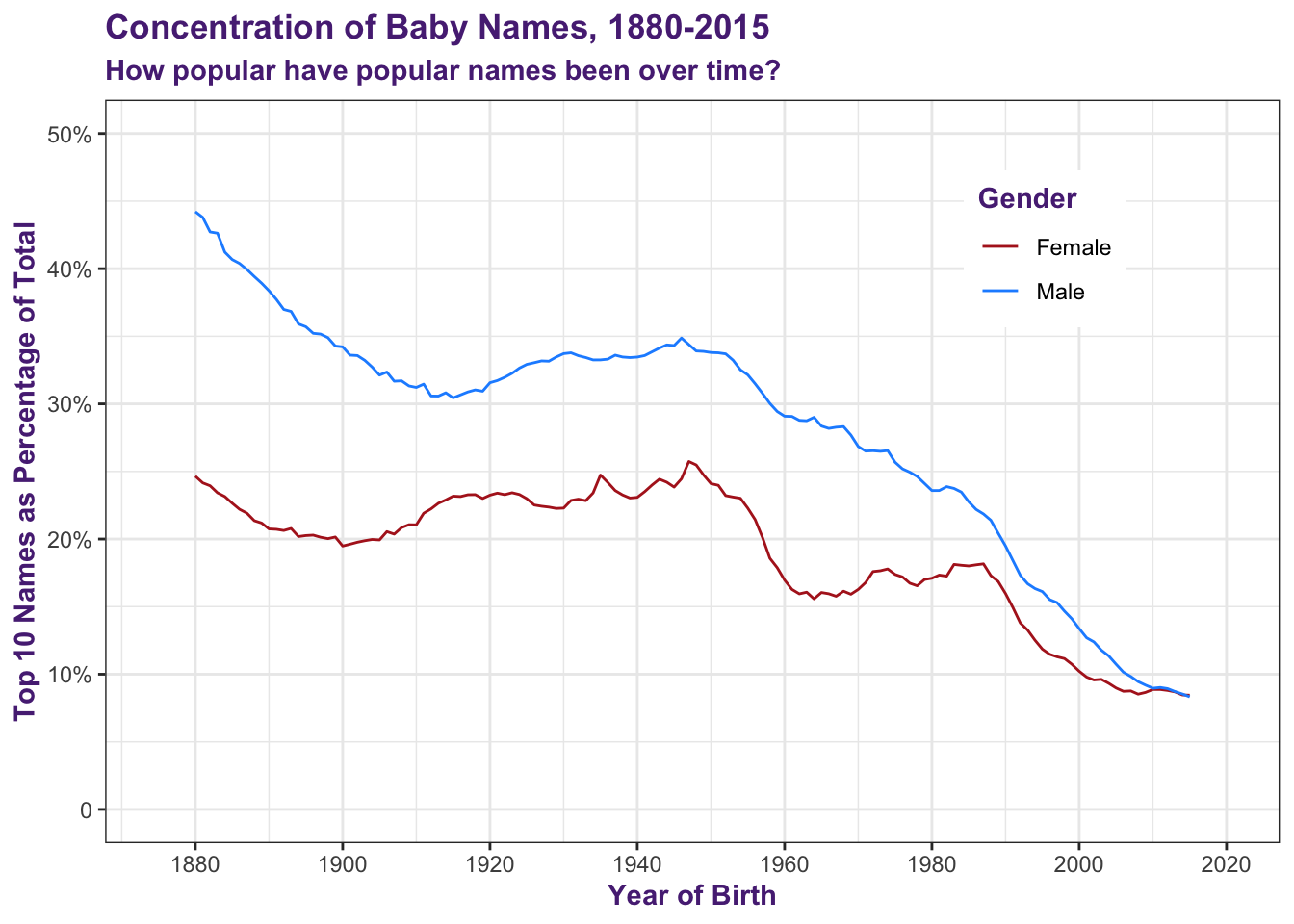
8 1883 M 1030 104627 44600One interesting calculation (among many) that we can perform on the data that we’ve gathered so far is to answer the following question: “How popular are the popular names for each sex in each year?” One way to answer this is to determine what percentage of all babies born each year have popular names. Let’s assume that “popular” means one of the top 10 names.
BabyYearSex <-
  BabyYearSex |>
    mutate(Concentration = CountTopBabiesThisYear / NumOfBabies)
head(BabyYearSex)
# A tibble: 6 × 6
# Groups: YearOfBirth [3]
YearOfBirth Sex NumOfNames NumOfBabies CountTopBabiesThisYear Concentration
<int> <chr> <int> <int> <int> <dbl>
1 1880 F 942 90992 22429 0.246
2 1880 M 1058 110490 48854 0.442
3 1881 F 938 91953 22211 0.242
4 1881 M 997 100743 44122 0.438
5 1882 F 1028 107848 25820 0.239
6 1882 M 1099 113686 48566 0.4274 Graphing
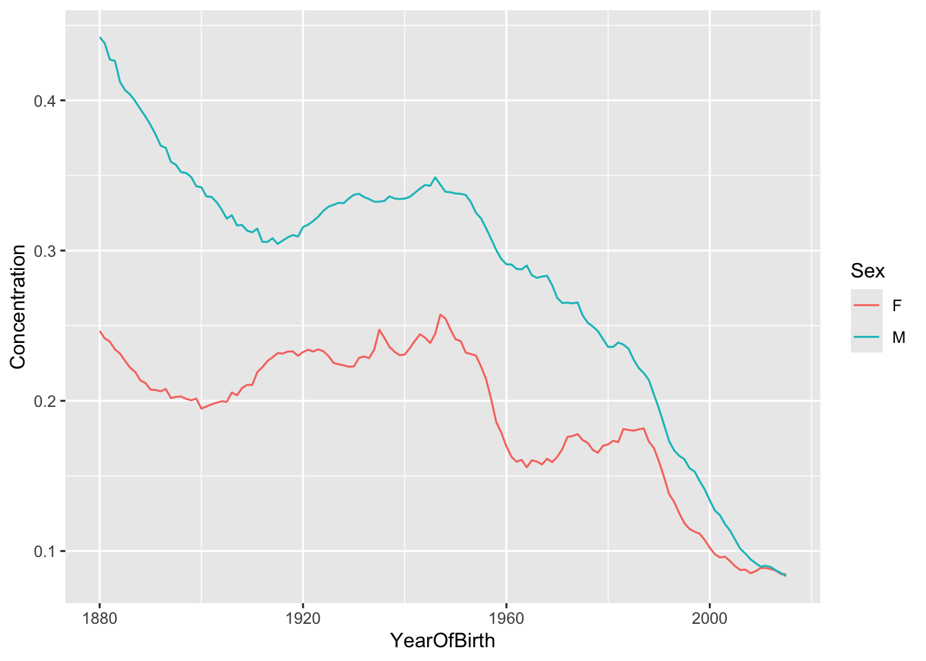
It’s pretty straight-forward to graph this in R (once you’ve gone through the graphing information for this class). Let’s do a basic version first:
We can see that since the mid 1940s, popular names have significantly dropped in popularity. Further, female names were much more concentrated in 1880 but are now on par with male names.
Now let’s do a little bit of design work:
BabyYearSex |>
  ggplot(aes(YearOfBirth, Concentration)) +
geom_line(aes(color = Sex)) +
scale_x_continuous(limits = c(1875, 2020),
breaks = c(1880, 1900, 1920, 1940, 1960, 1980, 2000, 2020)) +
scale_y_continuous(limits = c(0, 0.5),
breaks = c(0, 0.1, 0.2, 0.3, 0.4, 0.5),
labels = c("0", "10%", "20%", "30%", "40%", "50%")) +
scale_color_manual(values = c("F" = "firebrick", "M" = "dodgerblue"),
labels = c("Female", "Male")) +
labs(title = "Concentration of Baby Names, 1880-2015",
subtitle = "How popular have popular names been over time?",
x = "Year of Birth",
y = "Top 10 Names as Percentage of Total",
color = "Gender") +
theme_bw() +
theme(legend.position = c(0.8, 0.8),
title = element_text(colour = "#582C83",
face = "bold"))

